supply and demand paper assignment

Supply and Demand Paper Essay

Introduction, factors that can change supply and demand, substitutes of the product, complements of the product, how necessity impacts on the price elasticity of the product.

One of the most fundamental basics of micro-economics is the supply and demand of services or products of a given nature. Despite its frequent use, the analysis of the supply and demand of the products in the market provides a very basic understanding of the market nature and what should be done to promote either of the factors when it is down (John, 2001).

In every product that is in the market, one way or another there must be a substitute which is called competitor in the market and a complements which works together with the product, the most typical example of a complement is the ink of a biro pen, if you can buy a biro then you ought to afford the ink for the biro just like the case of a car and fuel, they are complements of each other even though they don’t have a direct relationship. The changes in the prices of one product can have some effects on the prices of its complements.

On the other hand, substitute products have a direct relationship because one can be replaced for the other. This effect is the genesis of the marketing strategies that we witness in the modern world. Increase in marketing strategies has been largely contributed by the increases in the number of the substitute products available in the market.

In essence, the higher the demand of a certain commodity or services, the higher the number of competitors in the market fighting for the commodity or the services by supplying the need to the market (John, 2006). This analysis is going to discuss the demand and the supply of a commodity which is the computer in this case.

Some of the factors that affect the demand and the supply of a computer include the following; the initial factor that can affect the supply of computer to a particular region is the demand of the computer services in the region.

If a region has less demand for computer services, there is going to be less demand for computers in the region. The supply of the computers is also limited by the availability of the substitute products like the PDA and advanced phone handsets that can perfectly perform the task of a computer.

Additionally, the demand of the computers is subject to the availability of services that requires computers, such activities includes the Cyber Café, computer learning center, major offices which computer systems required in a given region among other factors that will demand the services of computers.

In our case, some of the most common substitute of the computer includes; Personal Digital Assistant (PDA) and advanced mobile handsets. These two products are the major replacement or substitutes of the computer. They are the substitutes of the computer because one can use the product instead of opting to buy a computer.

A PDA is a typical example of a computer substitute because it does the functions of the computer with minimal effort and space unlike the computer which occupies space and hence creates inconvenience to the user while travelling. A mobile phone also creates a typical substitute of a computer because of its ability to perform the task of a computer with an added advantage of its size. The two products are the typical examples of the computer substitutes available in the market.

From the basics of microeconomics according to William (2008), a complement of a product is the product that is needed for the primary product to work properly. In essence, some of the most basic complements of a computer are the peripherals such as the printer, joysticks, scanners, the internet connection, and software systems.

There are both hardware and software complements of the computer. Software developers are usually the primary developers of the complements of a computer system. Software’s perform both the primary and the most fundamental role in a computer system; a computer cannot be functional without its software’s installed. Additionally, software’s perform the secondary factor of adding value to the computer system. The value added by the software’s has been the genesis of the ever increasing demand for the computer.

The elasticity in microeconomics as explained by John (2006) is the relative change in the demand with respect to the changes in the pricing of the commodity in question. It is usually expressed in a ratio as follows a typical graph for this ratio is normally given as shown below;

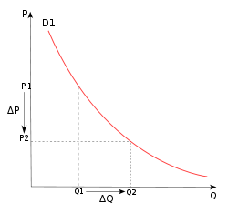
With the increase in the necessity of the product which is a computer in this case and keeping the price constant with other external factors, in an ideal situation, it is expected that the price elasticity of the of the computer will be positive.

In the real world this might not be the case because of the assumptions made; the increase in the necessity will lead to increase in the number of competitors who are substitutes of the product. On the other hand, the increase in the necessity may cause an increase in the price which may result in a constant or not effect on the elasticity of the product.

This paper has succinctly discussed the factors that influence the nature of the demands and the supply of a commodity which is taken to be a computer in this case. The demand of the computer is subject to its substitutes and to some extent its complements, it complements simply adds value to the computer while its substitutes reduces its demand in the market.

The price elasticity of the commodity is subject to the changes in demand as a ratio of the price. The necessity of the product is thus supposed to increase its price elasticity; however this is not always the case because of other influencing factors.

John, B. (2001). Economics: a student’s guide . Chicago, IL: Financial Times Prentice Hall.

John, T. (2006). Principles of Microeconomics . California, CA: Cengage Learning.

William, J., & Alan, S. (2008). Microeconomics: Principles and Policy . New York, NY: Cengage Learning.

• Chicago (A-D)
• Chicago (N-B)

IvyPanda. (2019, November 22). Supply and Demand Paper. https://ivypanda.com/essays/supply-and-demand-paper/

"Supply and Demand Paper." IvyPanda , 22 Nov. 2019, ivypanda.com/essays/supply-and-demand-paper/.

IvyPanda . (2019) 'Supply and Demand Paper'. 22 November.

IvyPanda . 2019. "Supply and Demand Paper." November 22, 2019. https://ivypanda.com/essays/supply-and-demand-paper/.

1. IvyPanda . "Supply and Demand Paper." November 22, 2019. https://ivypanda.com/essays/supply-and-demand-paper/.

Bibliography

IvyPanda . "Supply and Demand Paper." November 22, 2019. https://ivypanda.com/essays/supply-and-demand-paper/.

• Mobile and PDA Technologies Use in Education
• Strategic review for PDA Sim
• Apple Mobile Handset Improvement: Weather Resistance
• Operating Systems Used in Personal Digital Assistant (PDA)
• Future for mobile handsets in UK
• Patent Ductus Arteriosus: Symptoms/ Complaints
• Personal Digital Assistant Failure
• BlackBerry Handset in Arab World
• UniFirst and Progressive Insurance Corporation's Technologies
• Nokia Aims Way Beyond Handsets
• Monopolistic Competition as a Market Structure
• Economic Journal: Current Microeconomic Events
• Opportunity Cost in Microeconomics
• Principles of Macroeconomics: Supply and Demand Relationship
• Supply Cost Production and Profit

Want to create or adapt books like this? Learn more about how Pressbooks supports open publishing practices.

3 Supply and Demand

From Openstax Principles of Microeconomics (Chapter 3)

Economists use the term demand to refer to the amount of some good or service consumers are willing and able to purchase at each price. Demand is fundamentally based on needs and wants—if you have no need or want for something, you won’t buy it. While a consumer may be able to differentiate between a need and a want, but from an economist’s perspective, they are the same thing. Demand is also based on ability to pay. If you cannot pay for it, you have no effective demand. By this definition, a homeless person probably has no effective demand for shelter.

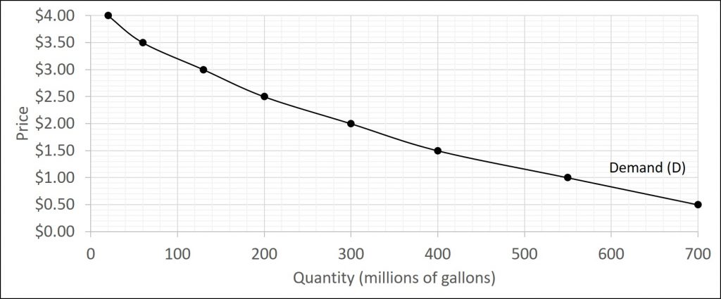
What a buyer pays for a unit of the specific good or service is called price. The total number of units that consumers would purchase at that price is called the quantity demanded. A rise in price of a good or service almost always decreases the quantity demanded of that good or service. Conversely, a fall in price will increase the quantity demanded. When the price of a gallon of gasoline increases, for example, people look for ways to reduce their consumption by combining several errands, commuting by carpool or mass transit, or taking weekend or vacation trips closer to home. Economists call this inverse relationship between price and quantity demanded the law of demand. The law of demand assumes that all other variables that affect demand (which we explain in the next module) are held constant.

We can show an example from the market for gasoline in a table or a graph. Economist call a table that shows the quantity demanded at each price, such as Table 3.1 below, a demand schedule. In this case, we measure price in dollars per gallon of gasoline. We measure the quantity demanded in millions of gallons over some time period (for example, per day or per year) and over some geographic area (like a state or a country). A demand curve shows the relationship between price and quantity demanded on a graph like the graph below, with quantity on the horizontal axis and the price per gallon on the vertical axis. (Note that this is an exception to the normal rule in mathematics that the independent variable (x) goes on the horizontal axis and the dependent variable (y) goes on the vertical. Economics is not math.)

The Law of Demand

Demand curves will appear somewhat different for each product. They may appear relatively steep or flat, or they may be straight or curved. Nearly all demand curves share the fundamental similarity that they slope down from left to right. Demand curves embody the law of demand: As the price increases, the quantity demanded decreases, and conversely, as the price decreases, the quantity demanded increases.

Demand versus Quantity Demanded

In economic terminology, demand is not the same as quantity demanded. When economists talk about demand, they mean the relationship between a range of prices and the quantities demanded at those prices, as illustrated by a demand curve or a demand schedule. When economists talk about quantity demanded, they mean only a certain point on the demand curve or one quantity on the demand schedule. In short, demand refers to the curve and quantity demanded refers to the (specific) point on the curve.

Individual and Market Demand

Shifts in demand.

The previous module explored how price affects the quantity demanded. The result was the demand curve. Price, however, is not the only factor that influences demand. For example, how is demand for vegetarian food affected if, say, health concerns cause more consumers to avoid eating meat? What are the major factors, in addition to the price, that influence demand?

We defined demand as the amount of some product a consumer is willing and able to purchase at each price. That suggests at least two factors in addition to price that affects demand. Willingness to purchase suggests a desire, based on what economists call tastes and preferences. If you neither need nor want something, you will not buy it. Ability to purchase suggests that income is important. Professors are usually able to afford better housing and transportation than students because they have more income. Prices of related goods can affect demand also. If you need a new car, the price of a Honda may affect your demand for a Ford. Finally, the size or composition of the population can affect demand. The more children a family has, the greater their demand for clothing. The more driving-age children a family has, the greater their demand for car insurance, and the less for diapers and baby formula.

These factors matter for both individual and market demand as a whole. Exactly how do these various factors affect demand, and how do we show the effects graphically? To answer those questions, we need the ceteris paribus assumption.

A demand curve is a relationship between two, and only two, variables: quantity on the horizontal axis and price on the vertical axis. The assumption behind a demand curve is that no relevant economic factors, other than the product’s price, are changing. Economists call this assumption ceteris paribus, a Latin phrase meaning “other things being equal.” Any given demand curve is based on the ceteris paribus assumption that all else is held equal. A demand curve  is a relationship between two, and only two, variables when all other variables are kept constant.

We will discuss a total of six factors which cause the demand curve to shift. You can use the mnemonic device INEPTT (which will be the same when we learn the supply shifters). These include:

• I ncome levels
• N umber of consumers
• E xpectations
• P rice of related goods

Each will be discussed in more depth shortly. Before we do that, let us explore what a change in demand actually is. Recall, when the price of a good changes, we move  along the demand curve. That is, when the price changes, the quantity demanded changes, but the demand stays the same (meaning we stay on the same demand curve.) On the other hand, when one of the shifters above changes, the entire demand curve moves. An increase in demand is shown by an outward shift while a decrease in demand is shown by an inward shift. This is shown graphically below.

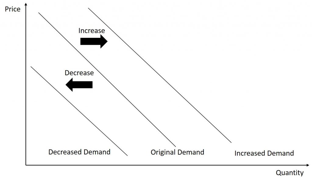
Numerically, what a shift means is that the quantity demanded will be different at each price level. The table below shows both an increase and decrease in demand using the demand schedule presented earlier in the chapter.

Now that we have explored what demand shifts look like, let us examine what can cause these changes.  Remember, if the price of the good changes, we move along the demand curve (meaning the demand curve does not move.)  It is only if one of the following factors change that the entire demand curve will move.

Changes in Income Levels

Consider the market for cars. Suppose that the market price of a car is $20,000. The original demand curve D, like every demand curve, is based on the ceteris paribus assumption that no other economically relevant factors change. Now imagine that the economy expands in a way that raises the incomes of many people, making cars more affordable. How will this affect demand?

The price of cars is still $20,000, but with higher incomes, the quantity demanded has now increased. As a result of the higher income levels, the demand curve shifts to the right to the new demand curve, indicating an increase in demand. This would occur at every price, not just the original one.

Now, imagine that the economy slows down so that many people lose their jobs or work fewer hours, reducing their incomes. In this case, the decrease in income would lead to a lower quantity of cars demanded at every given price, and the original demand curve would shift left. The shift represents a decrease in demand: At any given price level, the quantity demanded is now lower.

When a demand curve shifts, it does not mean that the quantity demanded by every individual buyer changes by the same amount. In this example, not everyone would have higher or lower income and not everyone would buy or not buy an additional car. Instead, a shift in a demand curve captures a pattern for the market as a whole.

The type of good just discussed is a normal good . That is, a good where if incomes rise the demand increases as well (and vice versa.) This is true for most goods and services. For some—luxury cars, vacations in Europe, and fine jewelry—the effect of a rise in income can be especially pronounced (we will discuss this in a later chapter).

A few exceptions to this pattern do exist. As incomes rise, many people will buy fewer generic brand groceries and more name brand groceries. They are less likely to buy used cars and more likely to buy new cars. They will be less likely to rent an apartment and more likely to own a home. A product whose demand falls when income rises, and vice versa, is called an inferior good . In other words, when income increases, the demand curve shifts to the left and vice versa.

Number of Consumers

This shifter is a bit more straightforward. This shifter is typically thought of as the population. Put simply, as the population of an area increases, the demand will increase and vice versa. This does not necessarily refer to the number of people interested in the product (this will be discussed later) but simply as the number of potential customers.

Expectations

While it is clear that the price of a good affects the quantity demanded, it is also true that expectations about the future price (or expectations about tastes and preferences, income, and so on) can affect demand. For example, if people hear that a hurricane is coming, they may rush to the store to buy flashlight batteries and bottled water. If people learn that the price of a good like coffee is likely to rise in the future, they may head for the store to stock up on coffee now. We show these changes in demand as shifts in the curve. Therefore, a shift in demand happens when a change in some economic factor (other than price) causes a different quantity to be demanded at every price.

Prices of Related Goods

Changes in the prices of related goods such as substitutes or complements also can affect the demand for a product. A substitute is a good or service that we can use in place of another good or service. As electronic books, like this one, become more available, you would expect to see a decrease in demand for traditional printed books. A lower price for a substitute decreases demand for the other product. For example, in recent years as the price of tablet computers has fallen, the quantity demanded has increased (because of the law of demand). Since people are purchasing tablets, there has been a decrease in demand for laptops, which we can show graphically as a leftward shift in the demand curve for laptops. A higher price for a substitute good has the reverse effect.

Other goods are complements for each other, meaning we often use the goods together because consumption of one good tends to enhance the consumption of the other. Examples include breakfast cereal and milk; notebooks and pens or pencils, golf balls and golf clubs; gasoline and sport utility vehicles; and the five-way combination of bacon, lettuce, tomato, mayonnaise, and bread. If the price of golf clubs rises, since the quantity demanded of golf clubs falls (because of the law of demand), demand for a complement good like golf balls decreases, too. Similarly, a higher price for skis would shift the demand curve for a complement good like ski resort trips to the left, while a lower price for a complement has the reverse effect.

This category contains several different components.

The first is changes in what consumers want. For instance, from 1980 to 2014, the per-person consumption of chicken by Americans rose from 48 pounds per year to 85 pounds per year, and consumption of beef fell from 77 pounds per year to 54 pounds per year, according to the U.S. Department of Agriculture (USDA). Changes like these are largely due to movements in taste, which change the quantity of a good demanded at every price: that is, they shift the demand curve for that good, rightward for chicken and leftward for beef. Similarly, fad items often see a rapid increase in demand when the item becomes popular and then a rapid shift inward when the item inevitably loses its popularity.

The second change is the demographics of an area. For example, the proportion of elderly citizens in the United States population is rising. It rose from 9.8% in 1970 to 12.6% in 2000 and will be a projected (by the U.S. Census Bureau) 20% of the population by 2030. A society with relatively more children, like the United States in the 1960s, will have greater demand for goods and services like tricycles and daycare facilities. A society with relatively more elderly persons, as the United States is projected to have by 2030, has a higher demand for nursing homes and hearing aids. Similarly, changes in the size of the population can affect the demand for housing and many other goods. Each of these changes in demand will be shown as a shift in the demand curve.

Taxes have the ability to impact a consumer’s ability to afford a good, but the type of tax impacts the change in demand.

Income taxes will affect demand in the same way as changes in income did because they are essentially the same thing. For instance, an increase in income tax means that people now have less disposable income. Therefore, an increase in income taxes will cause a decrease in the demand for normal goods and an increase in the demand for inferior goods.

A sales tax applied to each good equally will function the same way as the income tax. If you have to pay the same tax (as a percent of its price), your purchasing power is affected in the same way that an income tax affects your purchasing power.

On the other hand, an excise tax, which is a tax on a specific good, then there is movement along the demand curve for that good and not a shift in the entire curve. For instance, a pack of cigarettes may cost $5 but then a $3 tax is applied. The quantity demanded for a $5 pack of cigarettes is greater than the quantity demanded for an $8 pack of cigarettes.

The good news is that much of this section is similar, but in many cases opposite, to what we just learned.

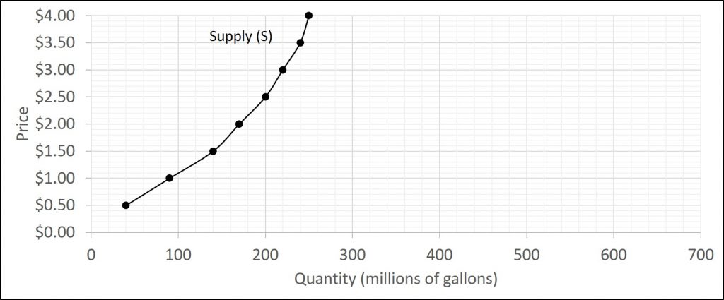
When economists talk about supply, they mean the amount of some good or service a producer is willing to supply at each price. Price is what the producer receives for selling one unit of a good or service. A rise in price almost always leads to an increase in the quantity supplied of that good or service, while a fall in price will decrease the quantity supplied. When the price of gasoline rises, for example, it encourages profit-seeking firms to take several actions: expand exploration for oil reserves; drill for more oil; invest in more pipelines and oil tankers to bring the oil to plants for refining into gasoline; build new oil refineries; purchase additional pipelines and trucks to ship the gasoline to gas stations; and open more gas stations or keep existing gas stations open longer hours. Economists call this positive relationship between price and quantity supplied—that a higher price leads to a higher quantity supplied and a lower price leads to a lower quantity supplied—the law of supply. The law of supply assumes that all other variables that affect supply are held constant.

The figure and table below both display the law of supply. Again, a supply schedule shows the different combinations of price and quantity supplied while the supply curve is a graphical representation of the same thing.

The Law of Supply

Supply curves will appear somewhat different for each product. They may appear relatively steep or flat, or they may be straight or curved. Nearly all supply curves share the fundamental similarity that they slope up from left to right. Supply curves embody the law of supply: As the price increases, the quantity supplied increases, and conversely, as the price decreases, the quantity supplied decreases.

Supply versus Quantity Supplied

In economic terminology, supply is not the same as quantity supplied. When economists talk about supply, they mean the relationship between a range of prices and the quantities supplied at those prices, as illustrated by a supply curve or a supply schedule. When economists talk about quantity supplied, they mean only a certain point on the supply curve, or one quantity on the supply schedule. In short, supply refers to the curve and quantity supplied refers to the (specific) point on the curve.

Individual and market supply

Shifts in supply.

The previous module explored how price affects the quantity supplied. The result was the supply curve. Price, however, is not the only factor that influences supply. For example, how is the supply of diamonds affected if diamond producers discover several new diamond mines? What are the major factors, in addition to the price, that influence supply?

These factors matter for both individual and market supply as a whole. Exactly how do these various factors affect supply, and how do we show the effects graphically? To answer those questions, we need the ceteris paribus assumption.

A supply curve is a relationship between two, and only two, variables: quantity on the horizontal axis and price on the vertical axis. The assumption behind a supply curve is that no relevant economic factors, other than the product’s price, are changing. Economists call this assumption ceteris paribus, a Latin phrase meaning “other things being equal.” Any given supply curve is based on the ceteris paribus assumption that all else is held equal. A supply curve is a relationship between two, and only two, variables when all other variables are kept constant.

We will discuss a total of six factors which cause the supply curve to shift. Again, notice INEPTT. These include:

• I nput prices (cost of production)
• N umber of suppliers
• P rice of alternative goods
• T echnology

Each will be discussed in more depth shortly. Before we do that, let us explore what a change in supply actually is. Recall, when the price of a good changes, we move  along the supply curve. That is, when the price changes, the quantity supplied changes, but the supply stays the same (meaning we stay on the same demand curve.) On the other hand, when one of the shifters above changes, the entire supply curve moves. An increase in supply is shown by an outward shift while a decrease in supply is shown by an inward shift. Be sure to think about shifts as inward or outward. If you think about the shift as moving the curve up or down, you will likely make mistakes with the supply curve. This is shown graphically below.

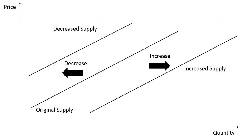
Numerically, what a shift means is that the quantity supplied will be different at each price level. The table below shows a both an increase and decrease in supply using the supply schedule presented earlier in the chapter.

Now that we have explored what supply shifts look like, let us examine what can cause these changes.  Remember, if the price of the good changes, we move along the supply curve (meaning the supply curve does not move.)  It is only if one of the following factors change that the entire supply curve will move.

Input Costs

A supply curve shows how quantity supplied will change as the price rises and falls, assuming ceteris paribus so that no other economically relevant factors are changing. If other factors relevant to supply do change, then the entire supply curve will shift. Just as we described a shift in demand as a change in the quantity demanded at every price, a shift in supply means a change in the quantity supplied at every price.

In thinking about the factors that affect supply, remember what motivates firms: profits, which are the difference between revenues and costs. A firm produces goods and services using combinations of labor, materials, and machinery, or what we call inputs or factors of production. If a firm faces lower costs of production, while the prices for the good or service the firm produces remain unchanged, a firm’s profits go up. When a firm’s profits increase, it is more motivated to produce output, since the more it produces the more profit it will earn. When costs of production fall, a firm will tend to supply a larger quantity at any given price for its output. We can show this by the supply curve shifting to the right.

Take, for example, a messenger company that delivers packages around a city. The company may find that buying gasoline is one of its main costs. If the price of gasoline falls, then the company will find it can deliver messages more cheaply than before. Since lower costs correspond to higher profits, the messenger company may now supply more of its services at any given price. For example, given the lower gasoline prices, the company can now serve a greater area and increase its supply.

Conversely, if a firm faces higher costs of production, then it will earn lower profits at any given selling price for its products. As a result, a higher cost of production typically causes a firm to supply a smaller quantity at any given price. In this case, the supply curve shifts to the left.

Imagine that the price of steel, an important ingredient in manufacturing cars, rises, so that producing a car has become more expensive. At any given price for selling cars, car manufacturers will react by supplying a lower quantity. We can show this graphically as a leftward shift of supply.

Conversely, if the price of steel decreases, producing a car becomes less expensive. At any given price for selling cars, car manufacturers can now expect to earn higher profits, so they will supply a higher quantity. The shift of supply to the right.

Number of Suppliers

This shifter is a bit more straightforward. This shifter is typically thought of as the number of firms. Put simply, as more firms enter the market, the supply will increase and vice versa.

Just as was the case with demand, firms will make decisions not only using current conditions but will also use expected changes to make decisions as well. For instance, if a firm expects the value of its product to increase in six months, they may temporarily decrease the amount of product they make available in order to make more of it available when the price goes up sometime in the future. For example, toy companies produce a significant amount of inventory throughout the year but do not make it available for sale until the holiday season. In addition, if a firm expects the cost of its inputs to rise, they may increase production today to avoid the higher cost of production that may occur later.

Price of Alternative Goods

Here we consider a single firm that produces more than one good. We know from the previous chapter that firms face a production possibilities frontier meaning that they can only produce so much given their factors of production. Therefore, the profitability of one good may impact the supply of another.

For example, consider a firm that produces widgets and gizmos. Now, suppose that the price of a widget increases. Since the price of the widget went up, the  quantity supplied of widgets will increase. But, in order to produce more widgets, the firm must shift some resources away from gizmo production. Therefore, the supply of gizmos decreases.

Be careful with terminology here. In the previous example, when the price of the widget changed, the quantity supplied of widgets changed, but the supply of gizmos changed. This is because the price of gizmos did not impact gizmo; instead, if was an external factor (in this case, the price of widgets) that affected production.

In summary, when the price of an alternative good (produced by the same firm) increases, the supply of the other good decreases and vice versa.

When a firm discovers a new technology that allows the firm to produce at a lower cost, the supply curve will shift to the right, as well. For instance, in the 1960s a major scientific effort nicknamed the Green Revolution focused on breeding improved seeds for basic crops like wheat and rice. By the early 1990s, more than two-thirds of the wheat and rice in low-income countries around the world used these Green Revolution seeds—and the harvest was twice as high per acre. A technological improvement that reduces costs of production will shift supply to the right so that a greater quantity will be produced at any given price.

Government policies can affect the cost of production and the supply curve through taxes, regulations, and subsidies. For example, the U.S. government imposes a tax on alcoholic beverages that collects about $8 billion per year from producers. Businesses treat taxes as costs. Higher costs decrease supply for the reasons we discussed above. Other examples of policy that can affect cost are the wide array of government regulations that require firms to spend money to provide a cleaner environment or a safer workplace. Complying with regulations increases costs.

A government subsidy, on the other hand, is the opposite of a tax. A subsidy occurs when the government pays a firm directly or reduces the firm’s taxes if the firm carries out certain actions. From the firm’s perspective, taxes or regulations are an additional cost of production that shifts supply to the left, leading the firm to produce a lower quantity at every given price. Government subsidies reduce the cost of production and increase supply at every given price, shifting supply to the right.

3.3 putting supply and demand together

Equilibrium.

Because the graphs for demand and supply curves both have price on the vertical axis and quantity on the horizontal axis, the demand curve and supply curve for a particular good or service can appear on the same graph. Together, demand and supply determine the price and the quantity that will be bought and sold in a market.

Remember this: When two lines on a diagram cross, this intersection usually means something. The point where the supply curve (S) and the demand curve (D) cross in the figure below is called the equilibrium. The equilibrium price is the only price where the plans of consumers and the plans of producers agree—that is, where the amount of the product consumers want to buy (quantity demanded) is equal to the amount producers want to sell (quantity supplied). Economists call this common quantity the equilibrium quantity. At any other price, the quantity demanded does not equal the quantity supplied, so the market is not in equilibrium at that price.

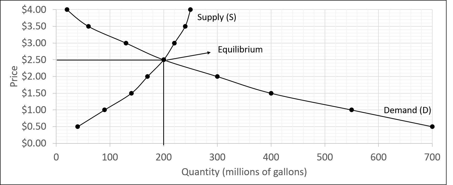
In the figure above, the equilibrium price is $2.50 per gallon of gasoline and the equilibrium quantity is 200 million gallons. If you had only the demand and supply schedules, and not the graph, you could find the equilibrium by looking for the price level on the tables where the quantity demanded and the quantity supplied are equal.

The word “equilibrium” means “balance.” If a market is at its equilibrium price and quantity, then it has no reason to move away from that point. However, if a market is not at equilibrium, then economic pressures arise to move the market toward the equilibrium price and the equilibrium quantity.

Market Failures

Imagine, for example, that the price of a gallon of gasoline was above the equilibrium price—that is, instead of $2.50 per gallon, the price is $3.00 per gallon. The horizontal line at the price of $3.00 in the figure below illustrates this above equilibrium price. At this higher price, the quantity demanded drops from 200 to 130. This decline in quantity reflects how consumers react to the higher price by finding ways to use less gasoline.

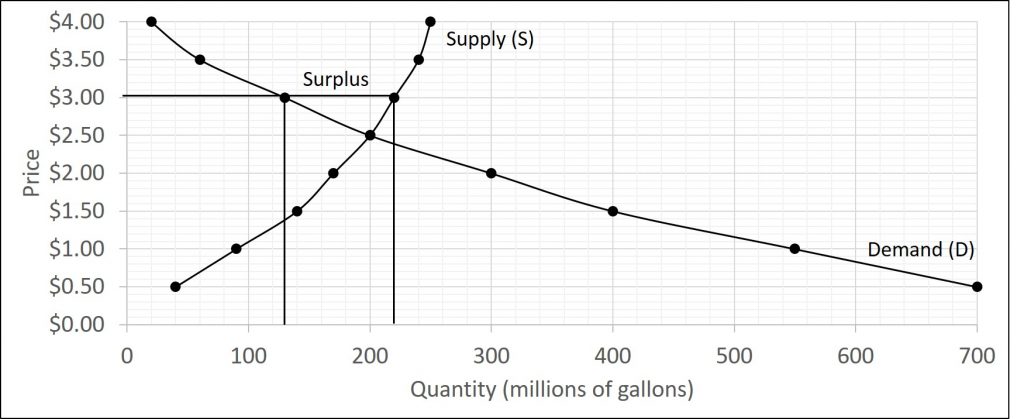
Moreover, at this higher price of $3.00, the quantity of gasoline supplied rises from the 200 to 220, as the higher price makes it more profitable for gasoline producers to expand their output. Now, consider how quantity demanded and quantity supplied are related at this above-equilibrium price. Quantity demanded has fallen to 130 gallons, while quantity supplied has risen to 220 gallons. In fact, at any above-equilibrium price, the quantity supplied exceeds the quantity demanded. We call this an excess supply or a surplus . In this example, the surplus is 220-130=90 million gallons.

With a surplus, gasoline accumulates at gas stations, in tanker trucks, in pipelines, and at oil refineries. This accumulation puts pressure on gasoline sellers. If a surplus remains unsold, those firms involved in making and selling gasoline are not receiving enough cash to pay their workers and to cover their expenses. In this situation, some producers and sellers will want to cut prices, because it is better to sell at a lower price than not to sell at all. Once some sellers start cutting prices, others will follow to avoid losing sales. These price reductions, in turn, will stimulate a higher quantity demanded. Therefore, if the price is above the equilibrium level, incentives built into the structure of demand and supply will create downward price pressure.

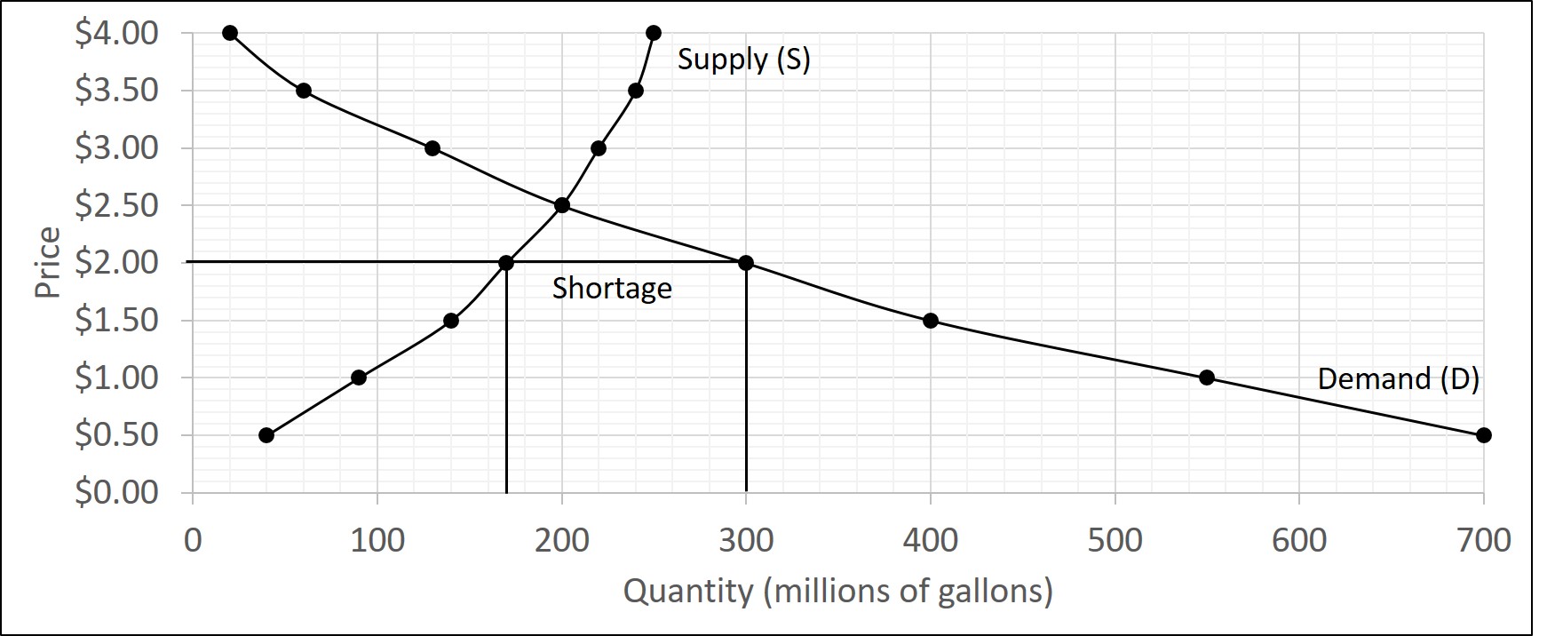
Now suppose that the price is below its equilibrium level at $2.00 per gallon, as the horizontal line at this price in Figure 3.7 shows. At this lower price, the quantity demanded increases from 200 to 300 as drivers take longer trips, spend more minutes warming up the car in the driveway in wintertime, stop sharing rides to work, and buy larger cars that get fewer miles to the gallon. However, the below-equilibrium price reduces gasoline producers’ incentives to produce and sell gasoline, and the quantity supplied falls from 200 to 170.

When the price is below equilibrium, there is excess demand, or a shortage —that is, at the given price the quantity demanded, which has been stimulated by the lower price, now exceeds the quantity supplied, which had been depressed by the lower price. In our example, the shortage is 300-170=130 millions of gallons. In this situation, eager gasoline buyers mob the gas stations, only to find many stations running short of fuel. Oil companies and gas stations recognize that they have an opportunity to make higher profits by selling what gasoline they have at a higher price. As a result, the price rises toward the equilibrium level.

Algebraic Equilibrium

Instead of using schedules or graphs to examine the supply and demand within a market, we can also express both as equations. This allows us to compact all of the information into a single mathematical expression. For instance, consider the demand equation below:

[latex]Q_{D}=30-5P.[/latex]

We can plug any price in and get the quantity demanded. For example, when the price is set at $3, the quantity demanded is

[latex]Q_{D}=30-5(3)=30-15=15.[/latex]

The same applies to the supply equation as well.

A market is in equilibrium when quantity demanded is equal to quantity supplied. Algebraically, this is accomplished by setting the demand equation equal to the supply equation. Then, you can solve for price. After you solve for price, you need to determine the equilibrium quantity. To accomplish this, plug the equilibrium price into either the demand or supply equation. To check your work, you can plug the equilibrium price into the other equation (depending on which equation you used first.) The quantities should be equal as this is the equilibrium condition (the quantity demanded must equal the quantity supplied.)

For example, let us find the equilibrium in the following market:

[latex]Q_{D}=30-5P[/latex]

[latex]Q_{S}=14+3P[/latex]

First, we set the equations equal:

[latex]Q_{D}=Q_{S}\Rightarrow 30-5P=14+3P[/latex]

Next, we solve for P:

[latex]30-5P+(-14+5P)=14+3P+(-14+5P) \Rightarrow 8P=16 \Rightarrow P=\frac{16}{8}[/latex]

Now, we plug the equilibrium price into the demand (or supply) equation:

[latex]Q_{D}=30-5(2)=30-10=20 \Rightarrow Q*=20.[/latex]

Finally, we can check our work by plugging the equilibrium price into the other equation. Since we used demand already, we will plug it into supply.

[latex]Q_{S}=14+3(2)=14+6=20 \Rightarrow Q*20.[/latex]

Therefore, the equilibrium price is $2 and the equilibrium quantity is 20 units.

Try the following problem: Find the equilibrium price and quantity in the following market:

[latex]Q_{D}=600-10P[/latex]

[latex]Q_{S}=200+15P[/latex]

[latex]Q_{D}=Q_{S}=600-10P=200+15P.[/latex]

Solving for P:

[latex]600-10P+(10P-200)=200+15P+(10P-200)\Rightarrow 25P=400[/latex]

[latex]\Rightarrow P=\frac{400}{25} \Rightarrow P^{*}=16.[/latex]

Plugging the equilibrium price into the demand equation:

[latex]Q_{D}=600-10(16)=440 \Rightarrow Q^{*}=440.[/latex]

Next, to check our work, we plug the equilibrium price in to the supply equation. We should get the same quantity.

[latex]Q_{S}=200+15(16)=440.[/latex]

Therefore, the equilibrium price is $16 and the equilibrium quantity is 440 units.

 We can also explore market failures algebraically as well. For example, consider the first example. What if the price in the market were set at $1.50. We can plug $1.50 into both the demand and supply equations:

[latex]Q_{D}=30-5(1.50)=22.5[/latex]

[latex]Q_{S}=14+3(1.50)=18.5[/latex]

Therefore, we face a shortage (since quantity supplied is less than quantity demanded) of 22.5-18.5=4 units.

3.4 Modeling market disequilibrium

Single shifts.

Let’s begin this discussion with a single economic event. It might be an event that affects demand, like a change in income, population, tastes, prices of substitutes or complements, or expectations about future prices. It might be an event that affects supply, like a change in natural conditions, input prices, or technology, or government policies that affect production. How does this economic event affect equilibrium price and quantity? We will analyze this question using a four-step process.

Step 1. Draw a demand and supply model before the economic change took place. To establish the model requires four standard pieces of information: The law of demand, which tells us the slope of the demand curve; the law of supply, which gives us the slope of the supply curve; the shift variables for demand; and the shift variables for supply. From this model, find the initial equilibrium values for price and quantity.

Step 2. Decide whether the economic change you are analyzing affects demand or supply. In other words, does the event refer to something in the list of demand factors or supply factors? Which specific factor is it affecting? Then, decide whether the effect on demand or supply causes the curve to shift to the right or to the left, and sketch the new demand or supply curve on the diagram. In other words, does the event increase or decrease the amount consumers want to buy or producers want to sell?

Step 3 . It is important to remember that in step 2, the only thing to change was the supply or demand. Therefore, coming into step 3, the price is still equal to the initial equilibrium price. Since either supply or demand changed, the market is in a state of disequilibrium. Thus, there is either a surplus or shortage. Determine which one exists. Next, determine what prices must do to reequilibrate the market. Remember, if there is a shortage, there will be upward price pressure and if there is a surplus, then there is downward price pressure. Prices continue to adjust until the market achieves a new equilibrium.

Step 4. Identify the new equilibrium and then compare the original equilibrium price and quantity to the new equilibrium price and quantity.

Example 1 (Supply)

Scenario: The market for fast food in a certain town is initially in equilibrium. Several new fast-food restaurants open in the town. Show the impact of the new fast-food restaurants on the equilibrium price and quantity of fast food in this town.

Step 1.  We begin by creating a supply and demand graph that is initially in equilibrium.

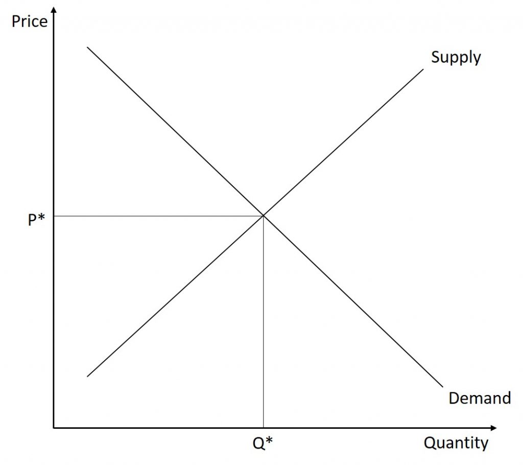
Step 2.  This change affects the supply of fast food. Specifically, the number of suppliers has increased. Therefore, the supply of fast food has increased. This causes an outward shift of the supply curve.

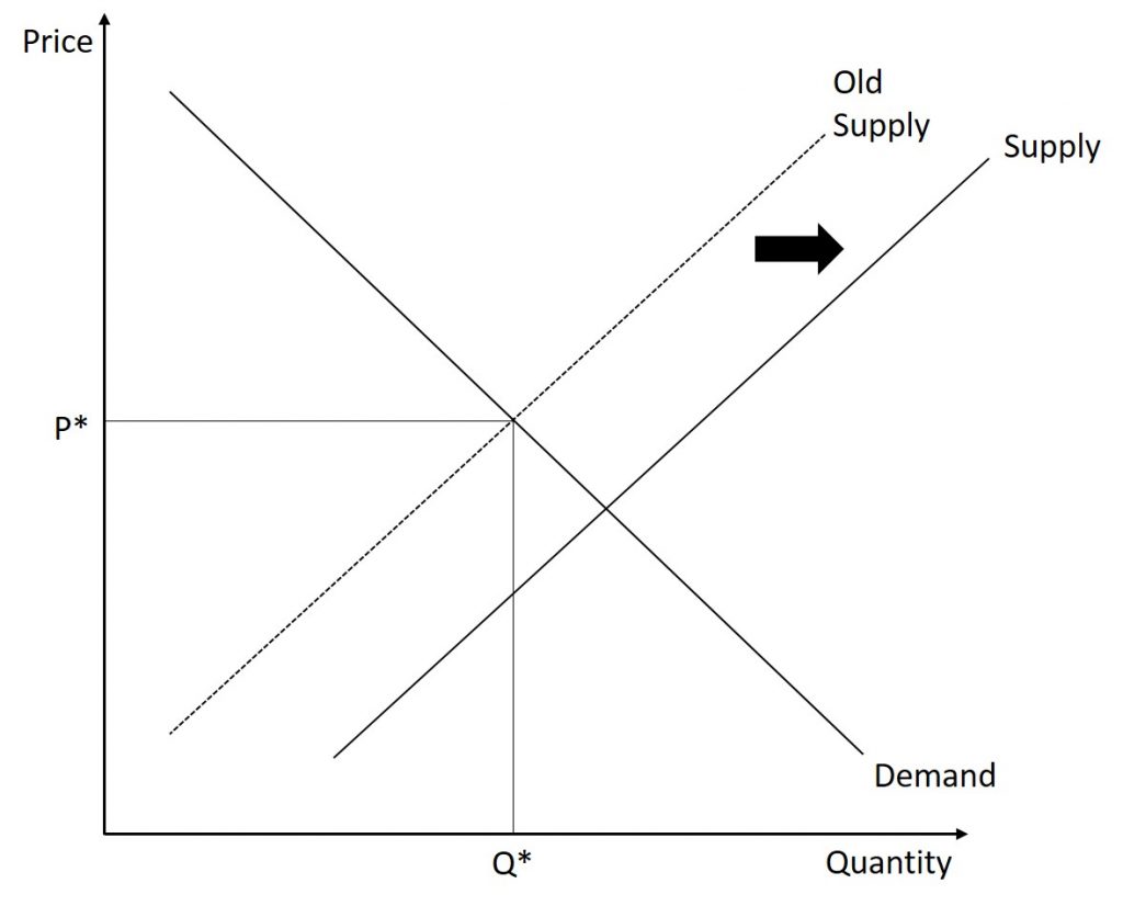
Step 3. At the original price level, the quantity demanded is less than the quantity supplied. Therefore, the market currently has a surplus. In order to alleviate the surplus, the price of fast food must begin to fall (downward price pressure.) This continues until the market achieves its new equilibrium.

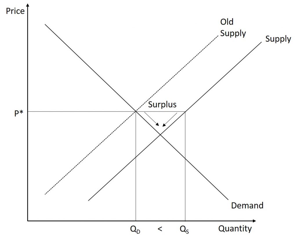
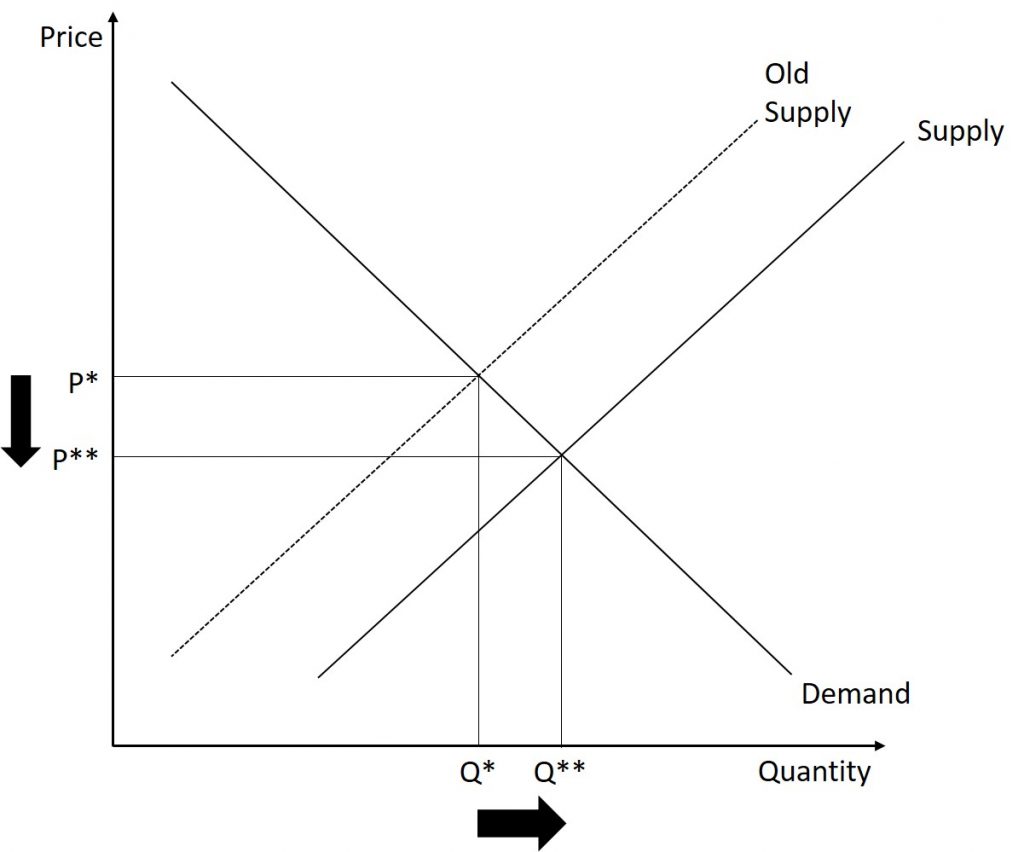
Step 4. We now compare the initial equilibrium to the new equilibrium. We can see that the price of fast food has fallen but the quantity of fast food has increased.

Example 2 (Demand)

Scenario: The market for pickup trucks is initially in equilibrium. A new marketing campaign is successful and creates a new desire to own pickup trucks. Show the impact of the advertising campaign on the equilibrium price and quantity of pickup trucks.

Step 2.  This change affects the demand for pickup trucks. Specifically, the tastes of consumers have changed. Therefore, the demand for pickup trucks has increased. This causes an outward shift of the demand curve.

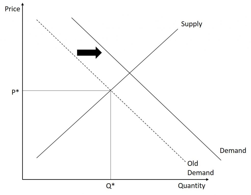
Step 3. At the original price level, the quantity supplied is less than the quantity demanded. Therefore, the market currently has a shortage. In order to alleviate the shortage, the price of pickup trucks will begin to increase (upward price pressure.) This continues until the market achieves its new equilibrium.

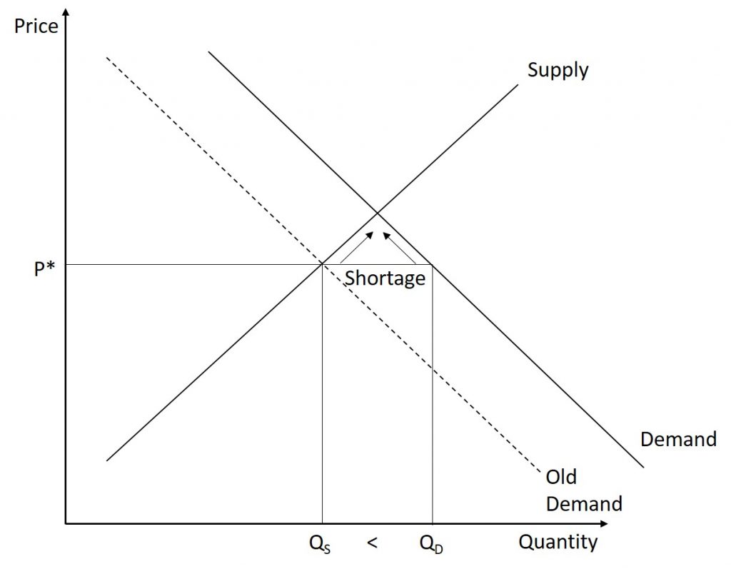
Step 4. We now compare the initial equilibrium to the new equilibrium. We can see that the price of pickup trucks has increased and the quantity of pickup trucks has increased.

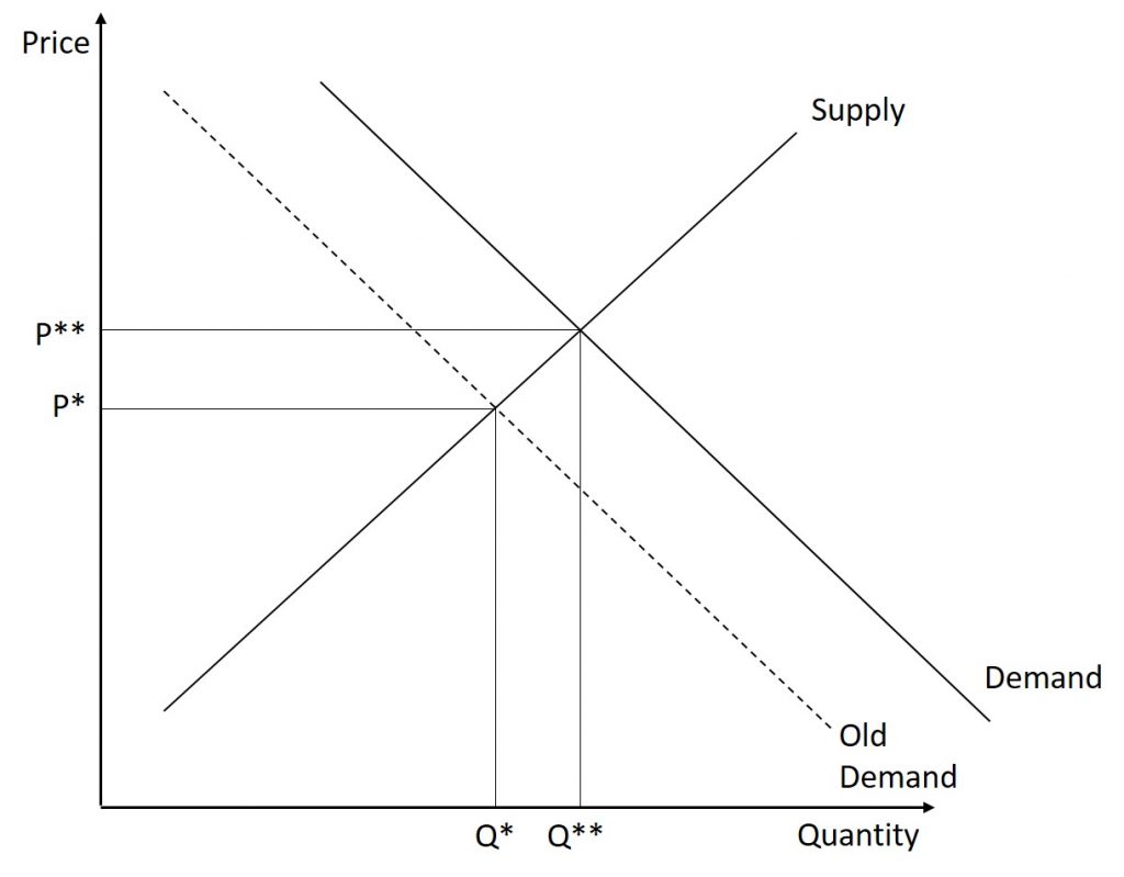
Summary of Shifts

Regardless of the cause of the shift, there are only a total of four possible cases. We can have an increase or decrease in supply or demand. Each scenario has its own unique template. The results are summarized below.

Double Shifts

In the previous examples, we examined the impact of a single change on the market. We saw that either supply or demand shifted (not both) and the curve only shifted once. But in reality, it is possible for several factors to change at the same time. Let us explore how we can model several changes within one graph.

The U.S. Postal Service is facing difficult challenges. Compensation for postal workers tends to increase most years due to cost-of-living increases. At the same time, increasingly more people are using email, text, and other digital message forms such as Facebook and Twitter to communicate with friends and others. What does this suggest about the continued viability of the Postal Service?

Instead of following the four-step procedure, let us think about the impact of each event separately. Then, we will put it on the same graph.

First, let us tackle increasing compensation. This can be considered as an input cost as labor is a required component of mail delivery. Recall that an increase in input costs will lead to a decrease in the supply. Thus, the supply curve will shift inward.

Next, let us tackle the change in the way people communicate. As people begin to use “snail-mail” less than ever, we can model the change as a decrease in the demand for mail service.

Let us put both of those shifts on the graph and determine what happens to the equilibrium price and quantity.

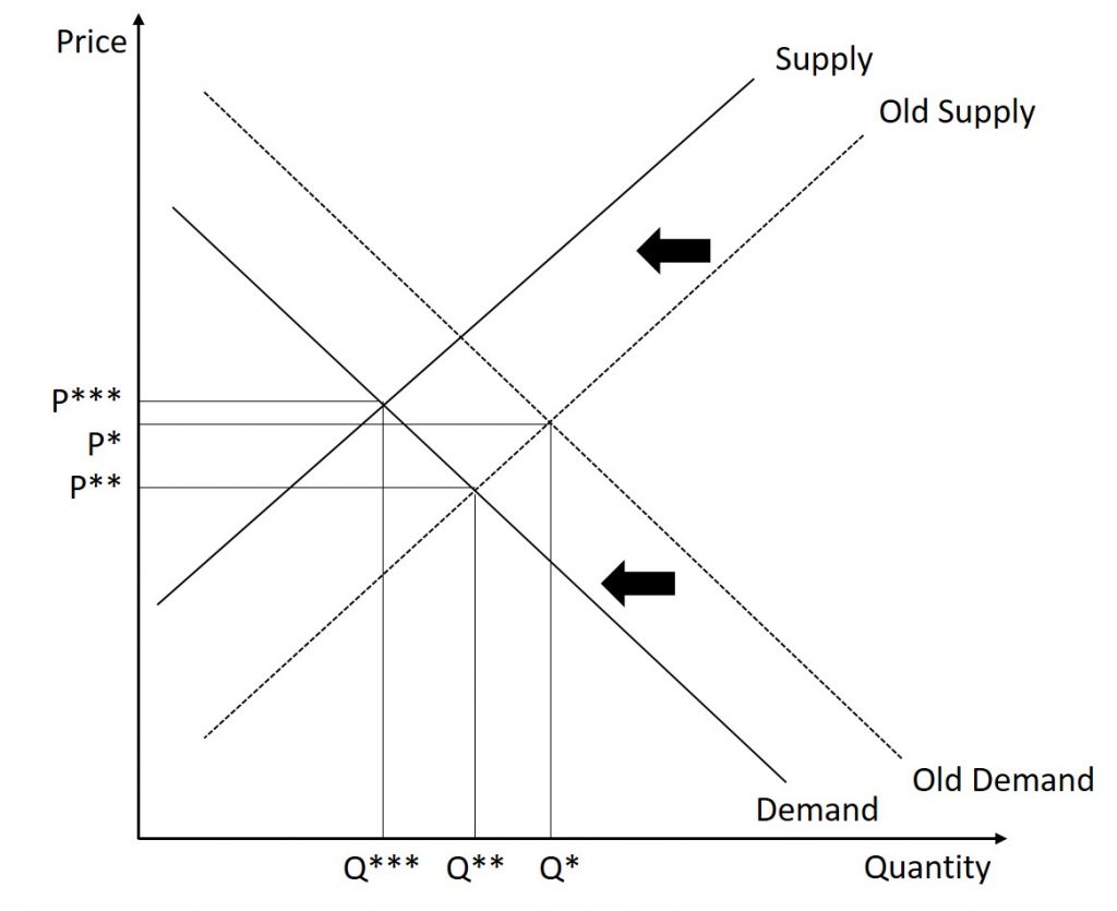
The inward shift of demand causes a decrease in both the equilibrium price and quantity. On the other hand, the decrease in supply causes an increase in the equilibrium price while it causes a decrease in the equilibrium quantity. Now, let us reconcile the two changes. The two changes caused both an increase and decrease in price. Therefore, there is no way for us to know the final impact on prices. The net effect is determined by which effect is larger (the demand shift versus the supply shift.) On the other hand, both shifts caused decreases in quantity. Therefore, we know there is a decrease in quantity. Thus, the net effect of the two shifts is an ambiguous change in price and a decrease in the equilibrium quantity.

3.5 Price controls

To this point in the chapter, we have been assuming that markets are free, that is, they operate with no government intervention. In this section, we will explore the outcomes, both anticipated and otherwise, when government does intervene in a market either to prevent the price of some good or service from rising “too high” or to prevent the price of some good or service from falling “too low”.

Economists believe there are a small number of fundamental principles that explain how economic agents respond in different situations. Two of these principles, which we have already introduced, are the laws of demand and supply.

Governments can pass laws affecting market outcomes, but no law can negate these economic principles. Rather, the principles will become apparent in sometimes unexpected ways, which may undermine the intent of the government policy. This is one of the major conclusions of this section. Controversy sometimes surrounds the prices and quantities established by demand and supply, especially for products that are considered necessities. In some cases, discontent over prices turns into public pressure on politicians, who may then pass legislation to prevent a certain price from climbing “too high” or falling “too low.”

The demand and supply model shows how people and firms will react to the incentives that these laws provide to control prices, in ways that will often lead to undesirable consequences. Alternative policy tools can often achieve the desired goals of price control laws while avoiding at least some of their costs and tradeoffs.

Price Ceilings

Laws that government enact to regulate prices are called price controls. Price controls come in two flavors. A price ceiling keeps a price from rising above a certain level (the “ceiling”), while a price floor keeps a price from falling below a given level (the “floor”). This section uses the demand and supply framework to analyze price ceilings. The next section discusses price floors.

A price ceiling is a legal maximum price that one pays for some good or service. A government imposes price ceilings in order to keep the price of some necessary good or service affordable. For example, in 2005 during Hurricane Katrina, the price of bottled water increased above $5 per gallon. As a result, many people called for price controls on bottled water to prevent the price from rising so high. In this particular case, the government did not impose a price ceiling, but there are other examples of where price ceilings did occur.

In many markets for goods and services, demanders outnumber suppliers. Consumers, who are also potential voters, sometimes unite behind a political proposal to hold down a certain price. In some cities, such as Albany, renters have pressed political leaders to pass rent control laws, a price ceiling that usually works by stating that landlords can raise rents by only a certain maximum percentage each year. Some of the best examples of rent control occur in urban areas such as New York, Washington D.C., or San Francisco.

Suppose that a city government passes a rent control law to keep the price at the original equilibrium of $500 for a typical apartment. In Figure 3.16, the horizontal line at the price of $500 shows the legally fixed maximum price set by the rent control law. The quantity demanded at $500 is 19,000 units while the quantity supplied is 15,000. Therefore, there is a shortage of 4,000 units when rent control is enforced. One of the ironies of price ceilings is that while the price ceiling was intended to help renters, there are actually fewer apartments rented out under the price ceiling (15,000 rental units) than would be the case at the market rent of $600 (17,000 rental units).

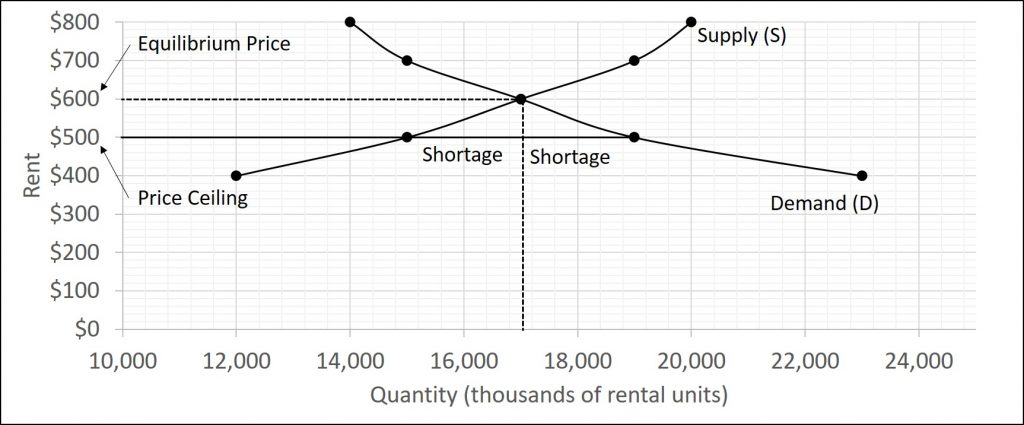
Price ceilings do not simply benefit renters at the expense of landlords. Rather, some renters (or potential renters) lose their housing as landlords convert apartments to co-ops and condos. Even when the housing remains in the rental market, landlords tend to spend less on maintenance and on essentials like heating, cooling, hot water, and lighting. The first rule of economics is you do not get something for nothing—everything has an opportunity cost. Thus, if renters obtain “cheaper” housing than the market requires, they tend to also end up with lower quality housing.

Price ceilings are enacted in an attempt to keep prices low for those who need the product. However, when the market price is not allowed to rise to the equilibrium level, quantity demanded exceeds quantity supplied, and thus a shortage occurs. Those who manage to purchase the product at the lower price given by the price ceiling will benefit, but sellers of the product will suffer, along with those who are not able to purchase the product at all. Quality is also likely to deteriorate.

Price ceilings can either be binding or non-binding. What has just be discussed is called a binding price ceiling since it prevents the market from achieving equilibrium. On the other hand, re-consider the last example. What if the price ceiling were set at $700? Some students believe that would cause the price to be set at $700 but this is incorrect. Remember, a price ceiling is just a legal maximum price. Therefore, a price ceiling of $700 only means that you cannot charge more than $700. So, even in the presence of the price ceiling, the market is able to achieve equilibrium. An important thing to keep in mind: if a market can achieve equilibrium, it will. The only time a price ceiling will have an impact on the market (that is, act as a binding price ceiling) is when the law makes the equilibrium price illegal.

Price Floor

A price floor is the lowest price that one can legally pay for some good or service. Perhaps the best-known example of a price floor is the minimum wage, which is based on the view that someone working full time should be able to afford a basic standard of living. The federal minimum wage in 2016 was $7.25 per hour, although some states and localities have a higher minimum wage. The federal minimum wage yields an annual income for a single person of$15,080, which is slightly higher than the federal poverty line of $11,880. As the cost of living rises over time, Congress periodically raises the federal minimum wage.

Price floors are sometimes called “price supports,” because they support a price by preventing it from falling below a certain level. Around the world, many countries have passed laws to create agricultural price supports. Farm prices and thus farm incomes fluctuate, sometimes widely. Even if, on average, farm incomes are adequate, some years they can be quite low. The purpose of price supports is to prevent these swings.

The most common way price supports work is that the government enters the market and buys up the product, adding to demand to keep prices higher than they otherwise would be. According to the Common Agricultural Policy reform passed in 2013, the European Union (EU) will spend about 60 billion euros per year, or 67 billion dollars per year (with the November 2016 exchange rate), or roughly 38% of the EU budget, on price supports for Europe’s farmers from 2014 to 2020.

Figure 3.17 illustrates the effects of a government program that assures a price above the equilibrium by focusing on the market for wheat in Europe. In the absence of government intervention, the price would adjust so that the quantity supplied would equal the quantity demanded at the equilibrium price. For this example, let us say that the free-market equilibrium price is $3.00 per bushel. However, policies to keep prices high for farmers keeps the price above what would have been the market equilibrium level—the price floor is shown by the dashed horizontal line in the diagram. For this example, let us say that is $4.00 per bushel. The result is a quantity supplied in excess of the quantity demanded (Qd). When quantity supplied exceeds quantity demanded, a surplus exists.

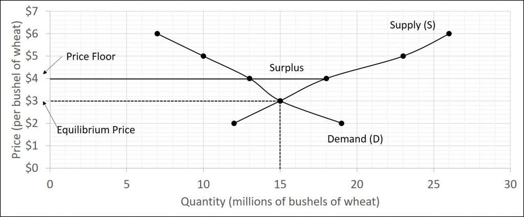
Economists estimate that the high-income areas of the world, including the United States, Europe, and Japan, spend roughly $1 billion per day in supporting their farmers. If the government is willing to purchase the excess supply (or to provide payments for others to purchase it)(also, there are times where the excess supply is simply destroyed), then farmers will benefit from the price floor, but taxpayers and consumers of food will pay the costs. Agricultural economists and policymakers have offered numerous proposals for reducing farm subsidies. In many countries, however, political support for subsidies for farmers remains strong. This is either because the population views this as supporting the traditional rural way of life or because of industry’s lobbying power of the agro-business.

Introduction to Microeconomics Copyright © 2019 by J. Zachary Klingensmith is licensed under a Creative Commons Attribution-ShareAlike 4.0 International License , except where otherwise noted.

Share This Book

Introduction to Demand and Supply

Chapter objectives.

In this chapter, you will learn about:

• Demand, Supply, and Equilibrium in Markets for Goods and Services
• Shifts in Demand and Supply for Goods and Services
• Changes in Equilibrium Price and Quantity: The Four-Step Process
• Price Ceilings and Price Floors

Bring It Home

Why can we not get enough of organic foods.

Organic food is increasingly popular, not just in the United States, but worldwide. At one time, consumers had to go to specialty stores or farmers' markets to find organic produce. Now it is available in most grocery stores. In short, organic has become part of the mainstream.

Ever wonder why organic food costs more than conventional food? Why, say, does an organic Fuji apple cost $2.75 a pound, while its conventional counterpart costs $1.72 a pound? The same price relationship is true for just about every organic product on the market. If many organic foods are locally grown, would they not take less time to get to market and therefore be cheaper? What are the forces that keep those prices from coming down? Turns out those forces have quite a bit to do with this chapter’s topic: demand and supply.

An auction bidder pays thousands of dollars for a dress Whitney Houston wore. A collector spends a small fortune for a few drawings by John Lennon. People usually react to purchases like these in two ways: their jaw drops because they think these are high prices to pay for such goods or they think these are rare, desirable items and the amount paid seems right.

Visit this website to read a list of bizarre items that have been purchased for their ties to celebrities. These examples represent an interesting facet of demand and supply.

When economists talk about prices, they are less interested in making judgments than in gaining a practical understanding of what determines prices and why prices change. Consider a price most of us contend with weekly: that of a gallon of gas. Why was the average price of gasoline in the United States $3.16 per gallon in June of 2020? Why did the price for gasoline fall sharply to $2.42 per gallon by January of 2021? To explain these price movements, economists focus on the determinants of what gasoline buyers are willing to pay and what gasoline sellers are willing to accept.

As it turns out, the price of gasoline in June of any given year is nearly always higher than the price in January of that same year. Over recent decades, gasoline prices in midsummer have averaged about 10 cents per gallon more than their midwinter low. The likely reason is that people drive more in the summer, and are also willing to pay more for gas, but that does not explain how steeply gas prices fell. Other factors were at work during those 18 months, such as increases in supply and decreases in the demand for crude oil.

This chapter introduces the economic model of demand and supply—one of the most powerful models in all of economics. The discussion here begins by examining how demand and supply determine the price and the quantity sold in markets for goods and services, and how changes in demand and supply lead to changes in prices and quantities.

As an Amazon Associate we earn from qualifying purchases.

This book may not be used in the training of large language models or otherwise be ingested into large language models or generative AI offerings without OpenStax's permission.

Want to cite, share, or modify this book? This book uses the Creative Commons Attribution License and you must attribute OpenStax.

Access for free at https://openstax.org/books/principles-economics-3e/pages/1-introduction

• Authors: Steven A. Greenlaw, David Shapiro, Daniel MacDonald
• Publisher/website: OpenStax
• Book title: Principles of Economics 3e
• Publication date: Dec 14, 2022
• Location: Houston, Texas
• Book URL: https://openstax.org/books/principles-economics-3e/pages/1-introduction
• Section URL: https://openstax.org/books/principles-economics-3e/pages/3-introduction-to-demand-and-supply

© Jan 23, 2024 OpenStax. Textbook content produced by OpenStax is licensed under a Creative Commons Attribution License . The OpenStax name, OpenStax logo, OpenStax book covers, OpenStax CNX name, and OpenStax CNX logo are not subject to the Creative Commons license and may not be reproduced without the prior and express written consent of Rice University.

If you're seeing this message, it means we're having trouble loading external resources on our website.

If you're behind a web filter, please make sure that the domains *.kastatic.org and *.kasandbox.org are unblocked.

To log in and use all the features of Khan Academy, please enable JavaScript in your browser.

Unit 2: Supply, demand, and market equilibrium

About this unit.

• Law of demand (Opens a modal)
• Market demand as the sum of individual demand (Opens a modal)
• Substitution and income effects and the law of demand (Opens a modal)
• Price of related products and demand (Opens a modal)
• Change in expected future prices and demand (Opens a modal)
• Changes in income, population, or preferences (Opens a modal)
• Normal and inferior goods (Opens a modal)
• Inferior goods clarification (Opens a modal)
• What factors change demand? (Opens a modal)
• Lesson summary: Demand and the determinants of demand (Opens a modal)
• Demand and the law of demand Get 5 of 7 questions to level up!
• Law of supply (Opens a modal)
• Change in supply versus change in quantity supplied (Opens a modal)
• Factors affecting supply (Opens a modal)
• What factors change supply? (Opens a modal)
• Lesson summary: Supply and its determinants (Opens a modal)
• Supply and the law of supply Get 3 of 4 questions to level up!

Market equilibrium and changes in equilibrium

• Market equilibrium (Opens a modal)
• Changes in market equilibrium (Opens a modal)
• Changes in equilibrium price and quantity when supply and demand change (Opens a modal)
• Changes in equilibrium price and quantity: the four-step process (Opens a modal)
• Lesson summary: Market equilibrium, disequilibrium, and changes in equilibrium (Opens a modal)
• Market equilibrium and disequilibrium Get 3 of 4 questions to level up!
• Changes in equilibrium Get 3 of 4 questions to level up!

• Search Search Please fill out this field.

Consumer Demand

Explaining supply, finding equilibrium, the bottom line.

• Macroeconomics

Introduction to Supply and Demand

The law of supply and demand is a fundamental concept of economics and a theory popularized by  Adam Smith  in 1776. The principles of supply and demand are effective in predicting market behavior. Whether an individual is a manufacturer or a consumer, the supply and demand equilibrium is relevant in daily market transactions.

Key Takeaways

• The law of supply and demand was popularized by Adam Smith in 1776.
• Consumer demand for a good commonly decreases as its price rises.
• As prices of a good increase, producers manufacture more to realize more profits.

Consumer demand for a good commonly decreases as its price rises. The figure below depicts the relationship between the price of a good and its demand from the consumer's standpoint. The demand curve is portrayed from the view of the consumer, whereas supply graphs are drawn from the producer's perspective.

If televisions were priced at $5 each, then consumers would purchase them and probably buy more TVs than they need based on price. The demand will remain high. If the price is $50,000, this good would likely be considered a luxury good , and demand would be low.

Demand is the quantity of a good that consumers are willing and able to purchase at various prices at a given time.

This example assumes that product differentiation does not exist. There is only one type of product sold at a single price to every consumer. In this closed scenario, the item is not an essential human necessity such as food or shelter, does not have a substitute, and consumers expect prices to remain stable. 

The supply curve considers the relationship between the price and available supply of an item from the producer's perspective rather than the consumer's.

When prices of a product increase, producers are willing to manufacture more of the product to realize greater profits. Falling prices depress production as producers may not recover input costs. If the costs to produce a TV are $50, production would be unprofitable when the selling price of the TV falls below $50.

If television prices are $1,000, manufacturers will focus on producing television sets over ventures and provide incentives to build more TVs. The behavior to seek maximum profits forces the supply curve to be upward-sloping. 

An underlying assumption of the theory lies in the producer taking on the role of a price taker. Rather than dictating the prices of the product, this input is determined by the market, and suppliers only face the decision of how much to produce, given the market price. Optimal scenarios are not always the case, such as in monopolistic markets.

Consumers typically look for the lowest cost, and producers test their products at the highest price. When prices become unreasonable, consumers change their preferences and move away from the product.

A proper balance must be achieved where both parties engage in ongoing business transactions to benefit consumers and producers. In supply and demand theory, the optimal price that results in producers and consumers achieving the maximum combined utility occurs where the supply and demand lines intersect.

In What Types of Economies Are Laws of Supply and Demand Less Reliable?

If the economic environment is not a free market, supply and demand are not influential factors. In  socialist economic systems , the government typically sets commodity prices regardless of the supply or demand conditions.

Does the Law of Supply and Demand Determine Market Conditions?

Multiple factors affect markets on both a microeconomic and a macroeconomic level. Supply and demand guide market behavior but do not determine it. Supply and demand are important factors, and Adam Smith referred to them as the  invisible hand  that guides a free market.

Does the Law of Supply and Demand Apply Only to Consumer Goods?

The theory of supply and demand relates not only to physical products such as television sets but also to wages and labor. More advanced theories of microeconomics and macroeconomics often adjust the assumptions and appearance of the supply and demand curve to illustrate concepts like economic surplus, monetary policy, aggregate supply and demand , fiscal stimulation, elasticity, and shortfalls.

The market theory of supply and demand was popularized by Adam Smith in 1776. Consumer demand for a good decreases as its price rises. As prices rise, producers manufacture more to gain more profits. The optimal price that shows an equilibrium between supply and demand is where the supply and demand lines intersect on a graph.

• A Practical Guide to Microeconomics 1 of 39
• Economists' Assumptions in Their Economic Models 2 of 39
• 5 Nobel Prize-Winning Economic Theories You Should Know About 3 of 39
• Positive vs. Normative Economics: What's the Difference? 4 of 39
• 5 Factors That Influence Competition in Microeconomics 5 of 39
• How Does Government Policy Impact Microeconomics? 6 of 39
• Microeconomics vs. Macroeconomics: What’s the Difference? 7 of 39
• How Do I Differentiate Between Micro and Macro Economics? 8 of 39
• Microeconomics vs. Macroeconomics Investments 9 of 39
• Introduction to Supply and Demand 10 of 39
• Is Demand or Supply More Important to the Economy? 11 of 39
• Demand: How It Works Plus Economic Determinants and the Demand Curve 12 of 39
• What Is the Law of Demand in Economics, and How Does It Work? 13 of 39
• Demand Curves: What Are They, Types, and Example 14 of 39
• Supply 15 of 39
• The Law of Supply Explained, With the Curve, Types, and Examples 16 of 39
• Supply Curve: Definition, How It Works, and Example 17 of 39
• Elasticity: What It Means in Economics, Formula, and Examples 18 of 39
• Price Elasticity of Demand: Meaning, Types, and Factors That Impact It 19 of 39
• Elasticity vs. Inelasticity of Demand: What's the Difference? 20 of 39
• What Is Inelastic? Definition, Calculation, and Examples of Goods 21 of 39
• What Affects Demand Elasticity for Goods and Services? 22 of 39
• What Factors Influence a Change in Demand Elasticity? 23 of 39
• Utility in Economics Explained: Types and Measurement 24 of 39
• Utility in Microeconomics: Origins, Types, and Uses 25 of 39
• Utility Function Definition, Example, and Calculation 26 of 39
• Definition of Total Utility in Economics, With Example 27 of 39
• Marginal Utilities: Definition, Types, Examples, and History 28 of 39
• What Is the Law of Diminishing Marginal Utility? With Example 29 of 39
• What Does the Law of Diminishing Marginal Utility Explain? 30 of 39
• Economic Equilibrium 31 of 39
• What Is the Income Effect? Its Meaning and Example 32 of 39
• Indifference Curves in Economics: What Do They Explain? 33 of 39
• Consumer Surplus Definition, Measurement, and Example 34 of 39
• What Is Comparative Advantage? 35 of 39
• What Are Economies of Scale? 36 of 39
• Perfect Competition: Examples and How It Works 37 of 39
• What Is the Invisible Hand in Economics? 38 of 39
• Market Failure: What It Is in Economics, Common Types, and Causes 39 of 39

• Terms of Service
• Editorial Policy
• Privacy Policy
• Your Privacy Choices

Browse Course Material

Course info.

• Prof. Jonathan Gruber

Departments

As taught in.

• Microeconomics

Learning Resource Types

Principles of microeconomics, problem set 1.

« Previous | Next »

Preparation

The problem set is comprised of challenging questions that test your understanding of the material covered in the course. Make sure you have mastered the concepts and problem solving techniques from the following sessions before attempting the problem set:

• Introduction to Microeconomics
• Applying Supply and Demand

Problem Set and Solutions

• Problem Set Questions (PDF)
• Problem Set Solutions (PDF)

Problem Solving Video

In the video below, a teaching assistant demonstrates his approach to the solution for problems 1 and 4 from the problem set. The teaching assistant notes common mistakes made by students and provides problem solving techniques for approaching similar questions on the problem set and exams.

• Download video
• Download transcript

You are leaving MIT OpenCourseWare

• school Campus Bookshelves
• menu_book Bookshelves
• perm_media Learning Objects
• login Login
• how_to_reg Request Instructor Account
• hub Instructor Commons
• Download Page (PDF)
• Download Full Book (PDF)
• Periodic Table
• Physics Constants
• Scientific Calculator
• Reference & Cite
• Tools expand_more
• Readability

selected template will load here

This action is not available.

6.24: Assignment- Problem Set — Supply and Demand

• Last updated
• Save as PDF
• Page ID 60653

Click on the link to download the problem set for this module:

• Supply and Demand Problem Set
• Supply and Demand Problem Set. Provided by : Lumen Learning. License : CC BY: Attribution

Aaron Smith

Are 231 - agricultural demand and supply.

The class is split in two halves. I cover supply in the first five weeks and Tim Beatty covers demand in the second five weeks. This page contains material from my part of the class.

I emphasize empirical work, but I do cover some applied theory. We start big and end small; the first topic is global agricultural supply and the last is field-level supply.

Syllabus:  2020 ,   2019

Blog Assignment

I post weekly Ag Data News  articles on my website that are loosely related to agricultural data. The articles are 600-1000 words with 3-4 figures. Your assignment is to write one of these articles.

Rules:       

• the topic must be something to do with agricultural supply
• you may work with a co-author
• you must provide code to generate any graphs that you create
• you may include graphs created by others (e.g., from papers, data portals such as FAOSTAT or my data apps .)

In 2020-2022, I published 8 student articles in Ag Data News. Follow this link and scroll to the bottom to read them.

Paper Assignments

These assignments require the students to do some empirical analysis to replicate and extend a paper, and to write up their work as though they aim to publish it in an academic journal. The papers must  not be more than five single-spaced pages (including tables and figures). I do not want the paper to read like a diary, i.e. “first I did this, then I did that”. Rather, I want them to tell a story, including an outline of the question they are asking, a discussion of the empirical method, the results, and a conclusion. A reader should be able to duplicate the analysis. 

1. Global food commodity supply

• Assignment (PDF)
• Basis of assignment:   Roberts, M.J., and W. Schlenker (2013) “ Identifying Supply and Demand Elasticities of Agricultural Commodities: Implications for the US Ethanol Mandate ,” American Economic Review 103: 2265–2295.

2. Climate change and agriculture (panel approach)

• Basis of assignment:   Fisher, A., M. Hanemann, M. Roberts, and W. Schlenker (2012) “ The economic impacts of climate change: evidence from agricultural output and random fluctuations in weather: comment ,” American Economic Review 102:3749–3760.

3. Climate change and agriculture (Ricardian approach)

• Basis of assignment:   Ortiz-Bobea, A. (2020) “ The Role of Nonfarm Influences in Ricardian Estimates of Climate Change Impacts on U.S. Agriculture, ” American Journal of Agricultural Economics . 102(3): 934-959.

4. Field-level supply

• Basis of assignment:   Hendricks, N.P, A. Smith, and D. Sumner (2015) “ Crop Supply Dynamics and the Illusion of Partial Adjustment ,” American Journal of Agricultural Economics, 96(5): 1469-1491.

Module 3: Supply and Demand

Assignment: problem set — supply and demand.

Step 1:  To view this assignment, click on  Assignment: Problem Set — Supply and Demand.

Contribute!

Improve this page Learn More

• Supply and Demand Problem Set. Provided by : Lumen Learning. License : CC BY: Attribution

Supply and Demand Simulation Paper Assignment

Supply and Demand Simulation Paper Principles of Microeconomics 365 Matthew J. Angner June 1, 2010 University of Phoenix Online Introduction The supply and demand simulation was based on the management of rental apartments by GoodLife Management. The apartments are in a fictitious town called Atlantis.

Topics that will be reviewed in this paper include changes in supply and demand, how shifts in supply and demand affects decision-making, key points from the reading assignments that were emphasized in the simulation, application of the supply and demand concepts at the author’s workplace, how price elasticity of demand affects the decision-making of the consumer and to the organization, and a summary of the results of the assessment. Causes for Change in Supply and Demand

Don’t waste your time! Order your assignment!

The causes for changes in supply and demand in the simulation were driven by the availability of two-bedroom rental apartment, demand for these rentals, the quantity of available renters, and the price per month. In the simulation, the demand curve is downward sloping so as the price of the rentals decreased, the demand increased. However, the supply curve is upward sloping. The number of apartments increased as the price increased. A surplus in the market for the apartments exerts downward pressure on the price. Adversely, a shortage in the market exerts an upward pressure on price.

To attract renters, GoodLife would need to lower prices if there were a surplus in the market or increase prices if there were a shortage in the market. In order to maintain the balance of quantity demanded and quantity supplied, GoodLife would need to raise their prices. Shifts in Supply and Demand Management directional changes of GoodLife along with population changes within Atlantis and the neighboring areas affected supply and demand. Preference changes of the tenants caused the demand for apartments to decrease. GoodLife management converted rental apartments into condominiums o sell causing a decrease in the supply causing a decrease in the supply and a decrease in demand at the same time. This created a shift to the left (decrease) in the supply curve and the demand curve. Key Points from Reading Assignments The four key points from the reading assignment emphasized in the simulation were supply and demand, equilibrium, shifts in supply and demand, and price ceilings. The simulation itself was based on the premise of supply and demand. Supply and demand is the economic term defining the relationship between demand, supply, and price. As price increases, quantity demanded decreases.

When price decreases, quantity demanded increases. Shifts in supply and demand were illustrated using different causes resulting in a decrease in supply and demand concurrently. Equilibrium is the quantity demanded equals the quantity supplied. When prices are below equilibrium, the quantity demanded exceeds the quantity supplied and there is a shortage in the market. Consumers, then, are willing to buy more than producers are willing to sell at this price. This causes price to increase. As price increases, quantity demanded decreases and quantity supplied increases.

This adjustment process continues until equilibrium is attained. Similarly, at prices above equilibrium, quantity supplied exceeds quantity demanded, and there is a surplus in the market. Producers are willing to sell more than consumers are willing to buy, which exerts a downward pressure on price. The price continues to decrease until equilibrium is attained. The simulation demonstrated that if apartment prices were below equilibrium, the number of apartments demanded exceeded the quantity available, which resulted in a shortage in the quantity of available apartments.

This also caused the price of the rental apartments to increase. If prices were above equilibrium, there would be a surplus of available apartments and this would drive the price down. Price ceilings are “a government imposed limit on how high a price can be charged” (Colander, 2008, p. 109). The limit is usually below the equilibrium price. Price ceilings can cause issues in the equilibrium between supply and demand. If the price for the apartments were at the ceiling price, and the demand for the apartments increase, the supply would then begin to decrease.

The simulation showed that this scenario escalated and the quantity demanded exceeded the quantity available and a shortage will continue. Application of Supply and Demand Concepts The writer has a career as a Supplier Development Engineer in the Automotive Industry. The products produced include interior and exterior door handles and exterior mirrors. Although there are other automotive supplier’s who produce the same products, generally there are only a handful of these suppliers. Therefore, understanding the market for the products produced affects production on a supply and demand level.

Changes in the economy in 2009 affected the production levels of our products. Vehicles were not selling, especially the larger SUV’s and truck platforms. Due to the decrease in demand, it created a surplus in the quantity of product on-hand. What did not occur, however, is a change in the price of the products. The product prices remained constant. What did change was the number of employees, which was reduced by 25% as well as a reduction in salaries for all employees. These reductions compensated for the pricing of the products not changing. Price Elasticity of Demand Price elasticity of demand is the percentage change in quantity demanded divided by the percentage change in price” (Colander, 2008, p. 128). It refers to the way prices change in relationship to the demand, or the way demand changes in relationship to price. Usually goods or services offered at a lower price leads to a demand for greater quantity. As a consumer, if an item is on sale, you may purchase several instead of just one. This means that though the seller offers the product at a lower price, he usually ends up making money because the demand for the product has increased.

However, if the price is too low, the retailer may lose money by selling too many at a reduced price. Results of Assessment The concepts of the supply and demand were the basis for the simulation on the management of rental apartments by GoodLife Management. The simulation demonstrated how different causes in supply and demand affected the availability of two-bedroom apartments and rental pricing. Key concepts covered included Supply and Demand, Equilibrium, Shifts in demand and supply, and price ceiling.

The application of supply and demand concepts at the author’s workplace were detailed as well as how price elasticity of demand can affect the decision-making process of the consumer and to an organization. References University of Phoenix. (2010). Applying Supply and Demand Concepts [Computer Software]. Retrieved from University of Phoenix, Simulation, ECO365 website. Colander, D. C. (2008). Economics 7th Edition. Retrieved from https://ecampus. phoenix. edu/content/eBookLibrary2/content/DownloadList. GRADE: 100%

How to cite this assignment

Related assignments:.

• Microeconomics And The Laws Of Supply And Demand Assignment
• Microeconomics and the Laws of Supply and Demand Assignment
• Microeconomics and the Law of Supply and Demand Assignment
• Analyzing Supply of Demand Simulation Assignment

Haven't Found The Paper You Want?

For Only $13.90/page

Assignment: Supply and Demand Paper Essay Example

• Pages: 4 (868 words)
• Published: March 15, 2017
• Type: Essay

I have had the personal experience of purchasing my college education. Picking a college was very challenging and I had huge amounts of pros and cons to weigh throughout my decision process. I knew that going to college and receiving a college education would be a wise investment and would better benefit me in the future financially. The supply and demand for a college education has changed over the years, thirty years ago a person might not have gone to college or paid for a college education and degree but that person still had a good chance of finding a steady job and becoming successful.

An example of this would be my father, he has worked for his company for forty years and he does not have a college education but he has become extremely successful within his company

. My father’s company now requires everyone that they hire to have a college education and at least an Associate degree but the company prefers for future employees to have a Bachelor degree. The factors that could cause possible changes in supply and demand for college would be the job demand, economy, technology, and the financial status that each person carries.

Job demands can be a cause of supply and demand due to the fact that many jobs do require their employees to have a college education and have knowledge of that particular field along with being trained. Many employees will want to move up in their job in order to get higher pay and to become more successful. At times it can be challenging to move up in a company without a college education and without a college

education employees tend to get paid less verses an employee who is college educated.

Economy has gotten worse and people depend on their jobs and incomes to pay bills and take care of their families, having a college education will help a person to make more money which means a earning a bigger income. Technology has become more advanced which means people need more education to fulfill their job duties and demands. The financial status that a person carries can often determine the supply and demand of receiving a college education due to the fact that if a person obtains a college education they would be able to make and earn more money.

Making more money is a plus but another factor to think about is school loans which will put a person in debt until the loans are paid off, so it is important for people to weigh their pros and cons when it comes to going to college. Now with the growing technology and job demands receiving a college education has increased in demand. People want to be successful in their careers and want a bigger income so a college education is the wisest way to become successful.

The supply for college is always elevated and increases each year because more and more people realize that receiving a college education is valuable and beneficial. Two substitutes for a college education would be self-educating which is where a person can get books, do research, and learn along with teaching themselves on a particular topic, business field, certain materials and information. Self-educating is what some people might prefer if they do not have the drive or determination, along

with finances to be able to go to college and earn a college degree.

Another substitute would be if a person would ask their job to sponsor or pay for classes, training, or even college courses to be able to have the opportunity to move up in the business and become more successful. Instead of receiving a college degree so companies will pay for their employees to earn college courses or training that will give them more knowledge and allow them to become more successful within the company. Two complements for a college education would be to first have a high school diploma or general education diploma then determine which degree to work towards such as an Associate, Bachelor, or Master degree.

Once receiving the desired level of education obtaining the desired job position would pay off for all of the hard work. The necessity of receiving a college education impacts price elasticity because the supply and demand for a college education is highly needed and seems to increase each year. I personally thought college was not for me and I would be just fine without a college education but after thinking about it I thought I would never get anywhere successful without a college education.

A good paying job requires a college education, the prices on everything rom cars, homes, and food increases each year. Receiving a college education is not only beneficial for me but also for my children, I am better to support them and be more accomplished and successful with a college education and degree. As the supply and demand increases each year for a college education so does the price of college educations.

Prices for a college education also vary depending on the career choice and degree that a person in working towards. Some professions and degrees take longer than others which of course cost more money.

• Benefits of a College Education Essay Example
• Should College Attendance Be Mandatory Essay Example
• Mr Burak Ceylan Essay Example
• University 101 Mid Semester Reflective Essay Example
• ArgumentativeEssay Essay
• College Essays
• Which Achievement In Our Lives Is Higher Than The Rest Essay Example
• Why Am I here Essay Example
• Only Educated Are Free Essay Example
• Analysis of 'Mid-Term Break' and 'Follower' Essay Example
• Mariah, by Che Husna Ashari Essay Example
• Practical Life - College Essay Example
• Effects of Playing dota Essay Example
• Termination of Agency Essay Example
• Engginering Essay Example
• Professor essays
• Should College be Free essays
• Should college athletes be paid essays
• College Education essays
• College Tuition essays
• Graduation essays
• College Goals essays
• Personal Statement essays
• Online Classes Vs Traditional Classes essays
• Online Education essays
• Student Loan essays
• Study Abroad Scholarship essays
• Reasons To Go To College essays
• Paying College Athletes essays
• Technology In The Classroom essays
• Academia essays
• Higher Education essays
• Language Learning essays
• Studying Business essays
• Education System essays
• Study essays
• First Day of School essays
• Scholarship essays
• Pedagogy essays
• Curriculum essays
• Coursework essays
• Studying Abroad essays
• Philosophy of Education essays
• Purpose of Education essays
• Brainstorming essays
• Educational Goals essays
• Importance Of College Education essays
• Brown V Board of Education essays
• The Importance Of Higher Education essays
• Online Education Vs Traditional Education essays
• Academic And Career Goals essays
• Academic Integrity essays
• Brown Vs Board Of Education essays
• Distance learning essays
• Technology in Education essays
• Vocabulary essays
• Writing Experience essays
• Importance of Education essays
• Early Childhood Education essays
• Academic Degree essays
• Academic Dishonesty essays
• School Uniform essays
• Academic writing essays
• Cheating essays
• Bachelor's Degree essays

Haven't found what you were looking for?

Search for samples, answers to your questions and flashcards.

• Enter your topic/question
• Receive an explanation
• Ask one question at a time
• Enter a specific assignment topic
• Aim at least 500 characters
• a topic sentence that states the main or controlling idea
• supporting sentences to explain and develop the point you’re making
• evidence from your reading or an example from the subject area that supports your point
• analysis of the implication/significance/impact of the evidence finished off with a critical conclusion you have drawn from the evidence.

Unfortunately copying the content is not possible

Tell us your email address and we’ll send this sample there..

By continuing, you agree to our Terms and Conditions .